Survival plots have never been so informative
Marcin Kosinski
Source:vignettes/Informative_Survival_Plots.Rmd
Informative_Survival_Plots.Rmd
This vignette covers changes between versions 0.1.0 and 0.2.0.
Motivation
Hadley Wickham’s ggplot2 version 2.0 revolution, at the end of 2015,
triggered many crashes in dependent R packages, that finally led to
deletions of few packages from The
Comprehensive R Archive Network. It occured that
survMisc package was removed from CRAN on 27th of January
2016 and R world remained helpless in the struggle with the elegant
visualizations of survival analysis. Then a new tool - survminer
package, created by Alboukadel
Kassambara - appeared on the R survival scene to fill the gap in
visualizing the Kaplan-Meier estimates of survival curves in elegant
grammar of graphics like way. This blog presents main features of core
ggsurvplot() function from survminer package, which
creates the most informative, elegant and flexible survival plots that I
have seen!
During the development of RTCGA package there was a need
to provide the simplest possible interface to estimates of survival
curves for biotechnologists and the
discovery of ggsurvplot() was a bull’s-eye! Many have
tried to provide a package or function for ggplot2-like plots that
would present the basic tool of survival analysis: Kaplan-Meier
estimates of survival curves, but none of earlier attempts have provided
such a rich structure of features and flexibility as survminer. On basis
of estimates of survival curves one can infere on differences in
survival times between compared groups, so survival plots are very
useful and can be seen in almost every publication in the field of
survival analysis and time to event models.
Example
After regular installation
install.packages('survminer')
BiocManager::install("RTCGA.clinical") # data for examples
we can create simple estimates of survival curves just after we put
survfit (survival package) object into
ggsurvplot() function. Let’s have a look at differences in
survival times between patients suffering from Ovarian Cancer
(Ovarian serous cystadenocarcinoma) and patients suffering from
Breast Cancer (Breast invasive carcinoma), where data were
collected by The
Cancer Genome Atlas Project.
library(survminer)
library(RTCGA.clinical)
survivalTCGA(BRCA.clinical, OV.clinical,
             extract.cols = "admin.disease_code") -> BRCAOV.survInfo
library(survival)
fit <- survfit(Surv(times, patient.vital_status) ~ admin.disease_code,
               data = BRCAOV.survInfo)
# Visualize with survminer
ggsurvplot(fit, data = BRCAOV.survInfo, risk.table = TRUE)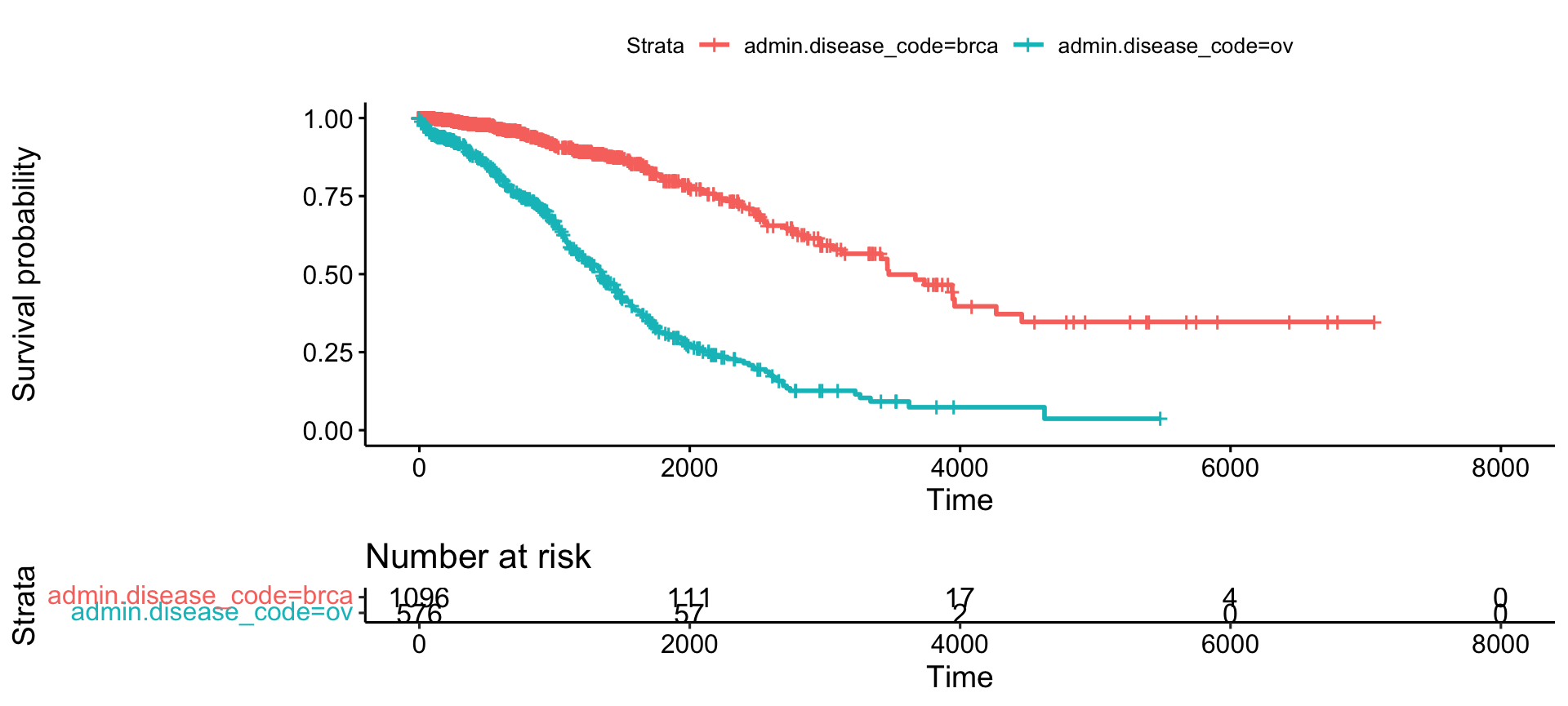
This simple plot presents, in an elegant way, estimates of survival probability depending on days from cancer diagnostics grouped by cancer types and an informative risk set table, which shows the number of patients that were under observation in the specific period of time. Survival analysis is a specific field of data analysis because of the censored time to event data, so risk set size is a must in visual inference.
After few improvements (#1, #2, #3, #4, #7, #8, #12, #28), made by Alboukadel in version 0.2.0, one can create a powerful, informative survival plot with such specification of parameters
ggsurvplot(
   fit,                     # survfit object with calculated statistics.
   data = BRCAOV.survInfo,  # data used to fit survival curves.
   risk.table = TRUE,       # show risk table.
   pval = TRUE,             # show p-value of log-rank test.
   conf.int = TRUE,         # show confidence intervals for
                            # point estimaes of survival curves.
   xlim = c(0,2000),        # present narrower X axis, but not affect
                            # survival estimates.
   break.time.by = 500,     # break X axis in time intervals by 500.
   ggtheme = theme_minimal(), # customize plot and risk table with a theme.
 risk.table.y.text.col = T, # colour risk table text annotations.
  risk.table.y.text = FALSE # show bars instead of names in text annotations
                            # in legend of risk table
)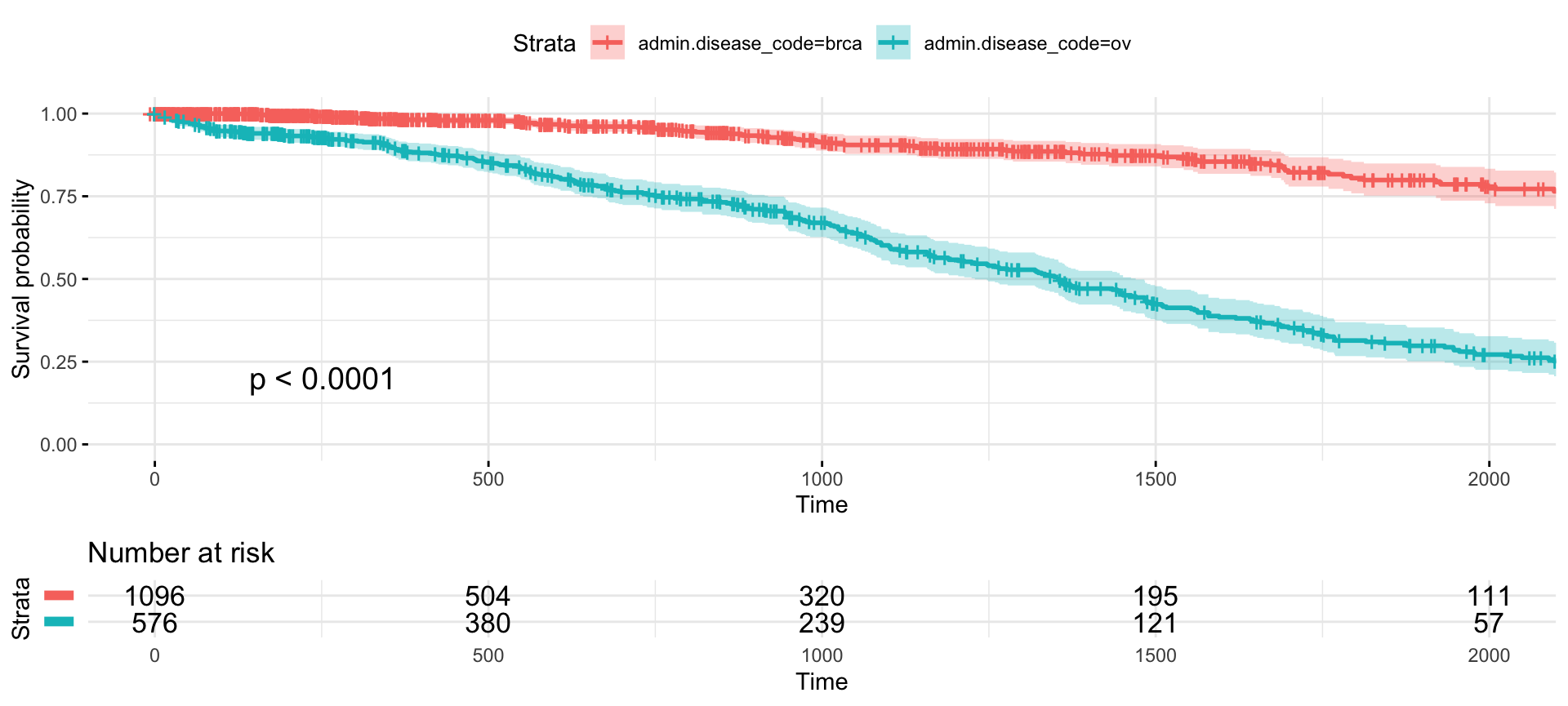
Each parameter is described in the correspoding comment, but I would
like to emphasize the xlim parameter which controls limits
of the X axis but does not affect the survival curves, that are taking
into account all possible times. Another brilliant parameter is
break.time.by that affects survival plots and the risk set
table - this would not be so easy to create it by yourself. Also a
ggtheme parameter is beneficial for simple plot
customization. Finally, risk.table.y.text and
risk.table.y.text.col (for which I have provided a user
requests) are useful parameters that change text (often too long and
redundand) from risk table legend into narrow, coloured bar. This saves
a lot of space in the final plot.
Comparisons
For comparison, below are survival curves obtained with the
base package.
base package
plot(fit) # base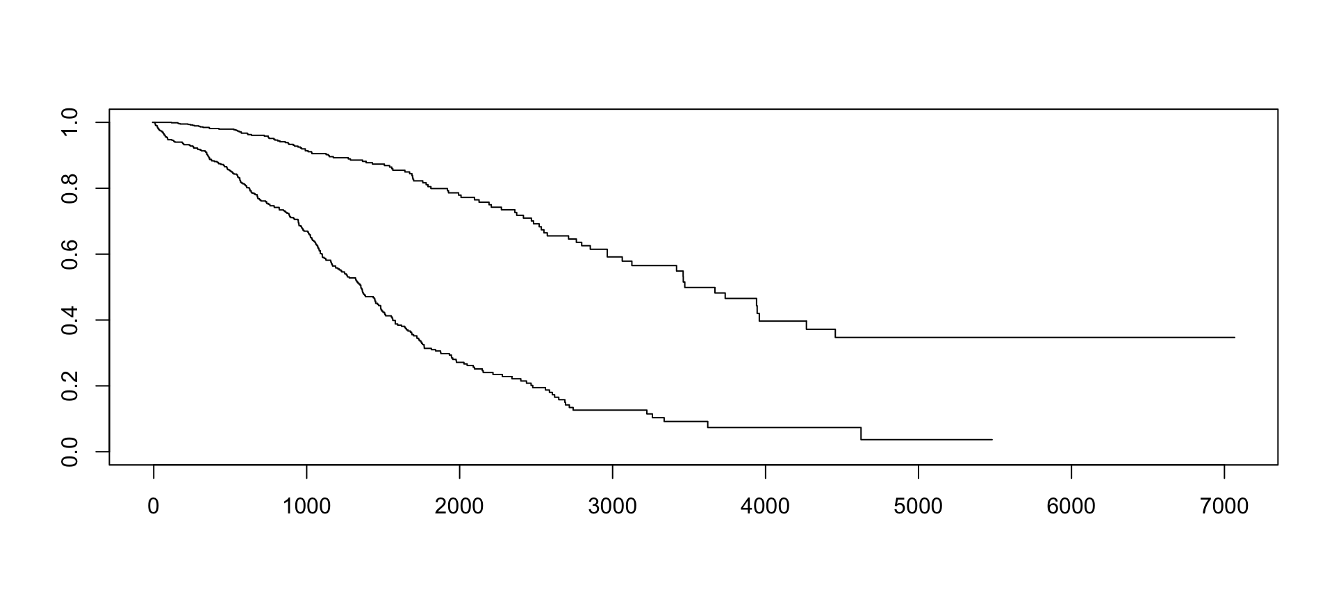
It looks pretty… base…
plot(fit, col=c("orange","purple"), lty=c(1:2), lwd=3, # base with some customization
     conf.int = TRUE, xmax = 2000)
# add a legend
legend(100, .2, c("Ovarian Cancer", "Breast Cancer"),
       lty = c(1:2), col=c("orange","purple"))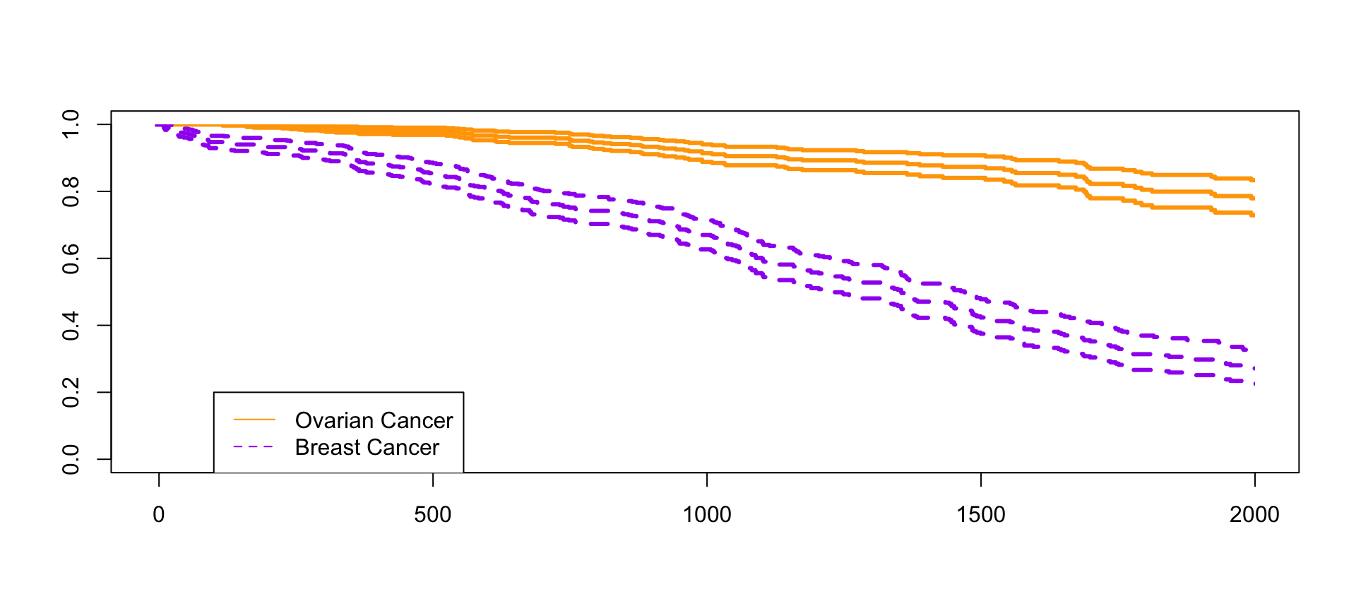
I haven’t seen examples with risk table and adding legend isn’t so quick as in survminer. Moreover, there are no minor axis breaks lines.
The
survminerpackage provides a much richer and more flexible interface for survival plots compared to base R graphics.