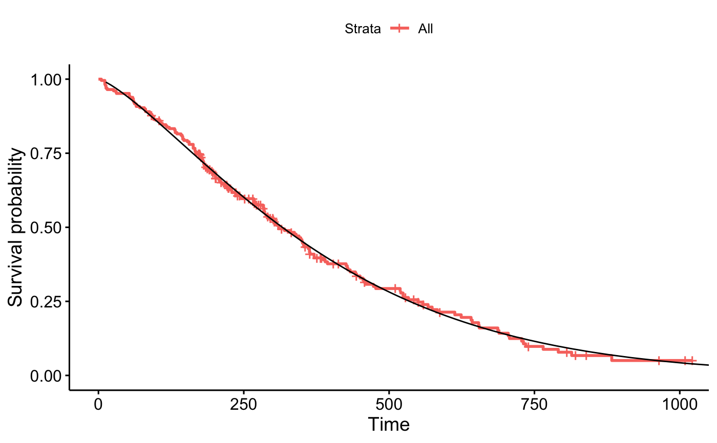
An extension to ggsurvplot() to plot survival curves from any data frame containing the summary of survival curves as returned the surv_summary() function.
Might be useful for a user who wants to use ggsurvplot for visualizing survival curves computed by another method than the standard survfit.formula function. In this case, the user has just to provide the data frame containing the summary of the survival analysis.
Usage
ggsurvplot_df(
  fit,
  fun = NULL,
  color = NULL,
  palette = NULL,
  linetype = 1,
  break.x.by = NULL,
  break.time.by = NULL,
  break.y.by = NULL,
  surv.scale = c("default", "percent"),
  surv.geom = geom_step,
  xscale = 1,
  conf.int = FALSE,
  conf.int.fill = "gray",
  conf.int.style = "ribbon",
  conf.int.alpha = 0.3,
  censor = TRUE,
  censor.shape = "+",
  censor.size = 4.5,
  title = NULL,
  xlab = "Time",
  ylab = "Survival probability",
  xlim = NULL,
  ylim = NULL,
  axes.offset = TRUE,
  legend = c("top", "bottom", "left", "right", "none"),
  legend.title = "Strata",
  legend.labs = NULL,
  ggtheme = theme_survminer(),
  ...
)
Arguments
- fit
a data frame as returned by surv_summary. Should contains at least the following columns:
time: survival time
surv: survival probability
strata: grouping variables
n.censor: number of censors
upper: upper end of confidence interval
lower: lower end of confidence interval
- fun
an arbitrary function defining a transformation of the survival curve. Often used transformations can be specified with a character argument: "event" plots cumulative events (f(y) = 1-y), "cumhaz" plots the cumulative hazard function (f(y) = -log(y)), and "pct" for survival probability in percentage.
- color
color to be used for the survival curves.
If the number of strata/group (n.strata) = 1, the expected value is the color name. For example color = "blue".
If n.strata > 1, the expected value is the grouping variable name. By default, survival curves are colored by strata using the argument color = "strata", but you can also color survival curves by any other grouping variables used to fit the survival curves. In this case, it's possible to specify a custom color palette by using the argument palette.
- palette
the color palette to be used. Allowed values include "hue" for the default hue color scale; "grey" for grey color palettes; brewer palettes e.g. "RdBu", "Blues", ...; or custom color palette e.g. c("blue", "red"); and scientific journal palettes from ggsci R package, e.g.: "npg", "aaas", "lancet", "jco", "ucscgb", "uchicago", "simpsons" and "rickandmorty". See details section for more information. Can be also a numeric vector of length(groups); in this case a basic color palette is created using the function palette.
- linetype
line types. Allowed values includes i) "strata" for changing linetypes by strata (i.e. groups); ii) a numeric vector (e.g., c(1, 2)) or a character vector c("solid", "dashed").
- break.x.by
alias of break.time.by. Numeric value controlling x axis breaks. Default value is NULL.
- break.time.by
numeric value controlling time axis breaks. Default value is NULL.
- break.y.by
same as break.x.by but for y axis.
- surv.scale
scale transformation of survival curves. Allowed values are "default" or "percent".
- surv.geom
survival curve style. Is the survival curve entered a step function (geom_step) or a smooth function (geom_line).
- xscale
numeric or character value specifying x-axis scale.
If numeric, the value is used to divide the labels on the x axis. For example, a value of 365.25 will give labels in years instead of the original days.
If character, allowed options include one of c("d_m", "d_y", "m_d", "m_y", "y_d", "y_m"), where d = days, m = months and y = years. For example, xscale = "d_m" will transform labels from days to months; xscale = "m_y", will transform labels from months to years.
- conf.int
logical value. If TRUE, plots confidence interval.
- conf.int.fill
fill color to be used for confidence interval.
- conf.int.style
confidence interval style. Allowed values include c("ribbon", "step").
- conf.int.alpha
numeric value specifying fill color transparency. Value should be in [0, 1], where 0 is full transparency and 1 is no transparency.
- censor
logical value. If TRUE, censors will be drawn.
- censor.shape
character or numeric value specifying the point shape of censors. Default value is "+" (3), a sensible choice is "|" (124).
- censor.size
numveric value specifying the point size of censors. Default is 4.5.
- title
main title
- xlab
x axis label
- ylab
y axis label
- xlim
x axis limits e.g.
xlim = c(0, 1000).- ylim
y axis limits e.g.
xlim = c(0, 1).- axes.offset
logical value. Default is TRUE. If FALSE, set the plot axes to start at the origin.
- legend
character specifying legend position. Allowed values are one of c("top", "bottom", "left", "right", "none"). Default is "top" side position. to remove the legend use legend = "none". Legend position can be also specified using a numeric vector c(x, y); see details section.
- legend.title
legend title.
- legend.labs
character vector specifying legend labels. Used to replace the names of the strata from the fit. Should be given in the same order as those strata.
- ggtheme
function, ggplot2 theme name. Default value is theme_survminer. Allowed values include ggplot2 official themes: see
theme.- ...
other arguments to be passed i) to ggplot2 geom_*() functions such as linetype, size, ii) or to the function ggpar() for customizing the plots. See details section.
Examples
library(survival)
# Fit survival curves
#::::::::::::::::::::::::::::::::::::::::::::::::::::::::
fit1 <- survfit( Surv(time, status) ~ 1, data = colon)
fit2 <- survfit( Surv(time, status) ~ adhere, data = colon)
# Summary
#::::::::::::::::::::::::::::::::::::::::::::::::::::::::
head(surv_summary(fit1, colon))
#> time n.risk n.event n.censor surv std.err upper lower
#> 1 8 1858 1 0 0.9994618 0.0005383580 1.0000000 0.9984077
#> 2 9 1857 1 0 0.9989236 0.0007615583 1.0000000 0.9974337
#> 3 19 1856 1 0 0.9983854 0.0009329660 1.0000000 0.9965614
#> 4 20 1855 1 0 0.9978471 0.0010775868 0.9999569 0.9957419
#> 5 23 1854 1 1 0.9973089 0.0012051037 0.9996673 0.9949561
#> 6 24 1852 1 1 0.9967704 0.0013206006 0.9993537 0.9941938
head(surv_summary(fit2, colon))
#> time n.risk n.event n.censor surv std.err upper lower
#> 1 8 1588 1 0 0.9993703 0.0006299213 1.0000000 0.9981372
#> 2 9 1587 1 0 0.9987406 0.0008911240 1.0000000 0.9969977
#> 3 19 1586 1 0 0.9981108 0.0010917438 1.0000000 0.9959774
#> 4 20 1585 1 0 0.9974811 0.0012610351 0.9999495 0.9950188
#> 5 23 1584 1 1 0.9968514 0.0014103253 0.9996107 0.9940997
#> 6 24 1582 1 1 0.9962213 0.0015455856 0.9992437 0.9932080
#> strata adhere
#> 1 adhere=0 0
#> 2 adhere=0 0
#> 3 adhere=0 0
#> 4 adhere=0 0
#> 5 adhere=0 0
#> 6 adhere=0 0
# Visualize
#::::::::::::::::::::::::::::::::::::::::::::::::::::::::
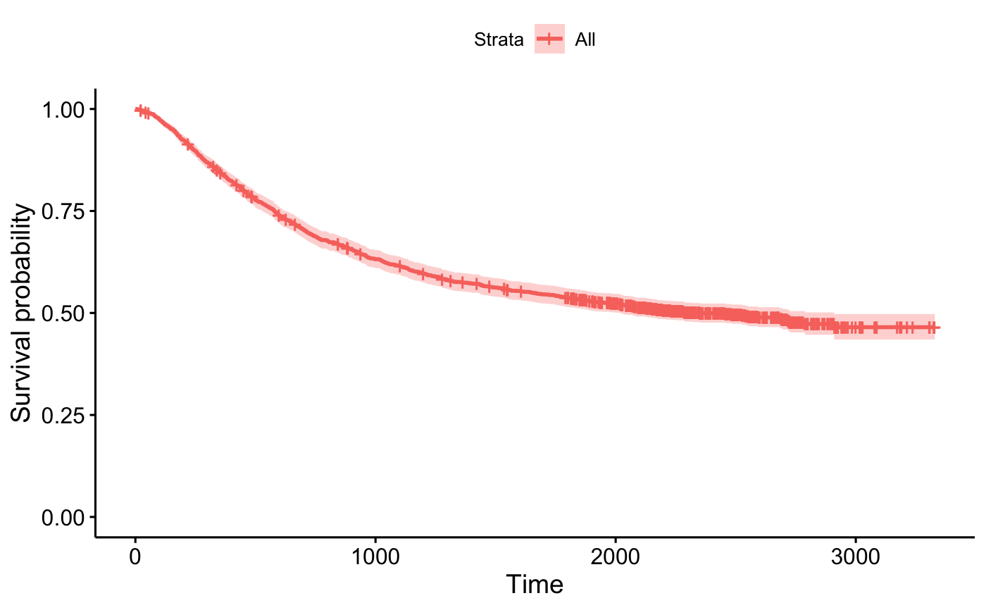
ggsurvplot_df(surv_summary(fit1, colon))
 ggsurvplot_df(surv_summary(fit2, colon), conf.int = TRUE,
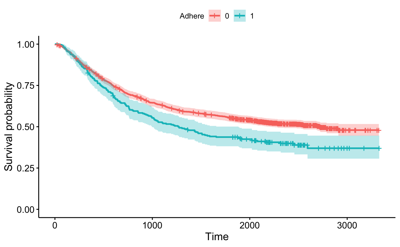
legend.title = "Adhere", legend.labs = c("0", "1"))
 # Kaplan-Meier estimate
#::::::::::::::::::::::::::::::::::::::::::::::::::::::::
out_km <- survfit(Surv(time, status) ~ 1, data = lung)
# Weibull model
#::::::::::::::::::::::::::::::::::::::::::::::::::::::::
wb <- survreg(Surv(time, status) ~ 1, data = lung)
s <- seq(.01, .99, by = .01)
t <- predict(wb, type = "quantile", p = s, newdata = lung[1, ])
out_wb <- data.frame(time = t, surv = 1 - s, upper = NA, lower = NA, std.err = NA)
# plot both
#::::::::::::::::::::::::::::::::::::::::::::::::::::::::
p_km <- ggsurvplot(out_km, conf.int = FALSE)
p_wb <- ggsurvplot(out_wb, conf.int = FALSE, surv.geom = geom_line)
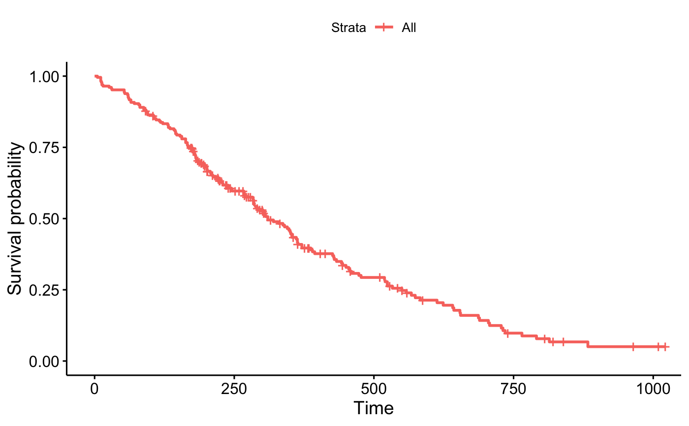
p_km
 p_wb
p_wb
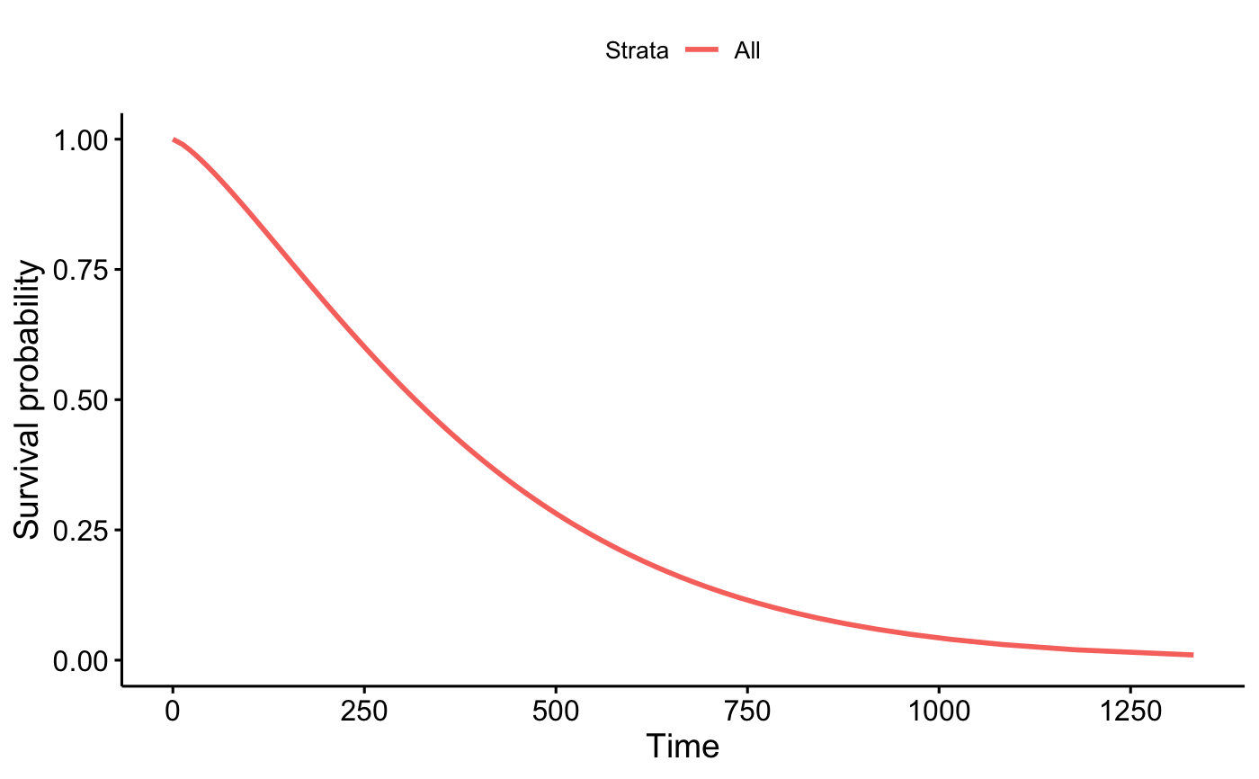 p_km$plot + geom_line(data = out_wb, aes(x = time, y = surv))
