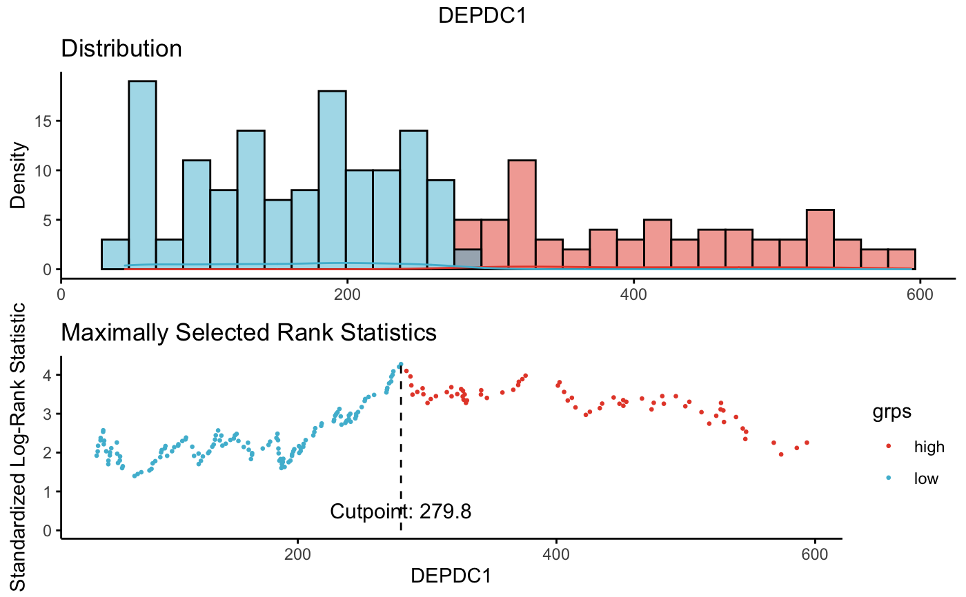
Determine the optimal cutpoint for one or multiple continuous variables at once, using the maximally selected rank statistics from the 'maxstat' R package. This is an outcome-oriented methods providing a value of a cutpoint that correspond to the most significant relation with outcome (here, survival).
surv_cutpoint(): Determine the optimal cutpoint for each variable using 'maxstat'.surv_categorize(): Divide each variable values based on the cutpoint returned bysurv_cutpoint().
Usage
surv_cutpoint(
  data,
  time = "time",
  event = "event",
  variables,
  minprop = 0.1,
  progressbar = TRUE
)

surv_categorize(x, variables = NULL, labels = c("low", "high"))

# S3 method for class 'surv_cutpoint'
summary(object, ...)

# S3 method for class 'surv_cutpoint'
print(x, ...)

# S3 method for class 'surv_cutpoint'
plot(x, variables = NULL, ggtheme = theme_classic(), bins = 30, ...)

# S3 method for class 'plot_surv_cutpoint'
print(x, ..., newpage = TRUE)
Arguments
- data
a data frame containing survival information (time, event) and continuous variables (e.g.: gene expression data).
- time, event
column names containing time and event data, respectively. Event values sould be 0 or 1.
- variables
a character vector containing the names of variables of interest, for wich we want to estimate the optimal cutpoint.
- minprop
the minimal proportion of observations per group.
- progressbar
logical value. If TRUE, show progress bar. Progressbar is shown only, when the number of variables > 5.
- x, object
an object of class surv_cutpoint
- labels
labels for the levels of the resulting category.
- ...
other arguments. For plots, see ?ggpubr::ggpar
- ggtheme
function, ggplot2 theme name. Default value is theme_classic. Allowed values include ggplot2 official themes. See
theme().- bins
Number of bins for histogram. Defaults to 30.
- newpage
open a new page. See
grid.arrange.
Value
surv_cutpoint(): returns an object of class 'surv_cutpoint', which is a list with the following components:
maxstat results for each variable (see ?maxstat::maxstat)
cutpoint: a data frame containing the optimal cutpoint of each variable. Rows are variable names and columns are c("cutpoint", "statistic").
data: a data frame containing the survival data and the original data for the specified variables.
minprop: the minimal proportion of observations per group.
not_numeric: contains data for non-numeric variables, in the context where the user provided categorical variable names in the argument variables.
surv_categorize(): returns an object of class 'surv_categorize', which is a data frame containing the survival data and the categorized variables.
Author
Alboukadel Kassambara, alboukadel.kassambara@gmail.com
Examples
# 0. Load some data
data(myeloma)
head(myeloma)
#>          molecular_group chr1q21_status treatment event  time   CCND1 CRIM1
#> GSM50986      Cyclin D-1       3 copies       TT2     0 69.24  9908.4 420.9
#> GSM50988      Cyclin D-2       2 copies       TT2     0 66.43 16698.8  52.0
#> GSM50989           MMSET       2 copies       TT2     0 66.50   294.5 617.9
#> GSM50990           MMSET       3 copies       TT2     1 42.67   241.9  11.9
#> GSM50991             MAF           <NA>       TT2     0 65.00   472.6  38.8
#> GSM50992    Hyperdiploid       2 copies       TT2     0 65.20   664.1  16.9
#>          DEPDC1    IRF4   TP53   WHSC1
#> GSM50986  523.5 16156.5   10.0   261.9
#> GSM50988   21.1 16946.2 1056.9   363.8
#> GSM50989  192.9  8903.9 1762.8 10042.9
#> GSM50990  184.7 11894.7  946.8  4931.0
#> GSM50991  212.0  7563.1  361.4   165.0
#> GSM50992  341.6 16023.4 2096.3   569.2

# 1. Determine the optimal cutpoint of variables
res.cut <- surv_cutpoint(myeloma, time = "time", event = "event",
   variables = c("DEPDC1", "WHSC1", "CRIM1"))

summary(res.cut)
#>        cutpoint statistic
#> DEPDC1    279.8  4.275452
#> WHSC1    3205.6  3.361330
#> CRIM1      82.3  1.968317

# 2. Plot cutpoint for DEPDC1
# palette = "npg" (nature publishing group), see ?ggpubr::ggpar
plot(res.cut, "DEPDC1", palette = "npg")
#> $DEPDC1

#>

# 3. Categorize variables
res.cat <- surv_categorize(res.cut)
head(res.cat)
#>           time event DEPDC1 WHSC1 CRIM1
#> GSM50986 69.24     0   high   low  high
#> GSM50988 66.43     0    low   low   low
#> GSM50989 66.50     0    low  high  high
#> GSM50990 42.67     1    low  high   low
#> GSM50991 65.00     0    low   low   low
#> GSM50992 65.20     0   high   low   low

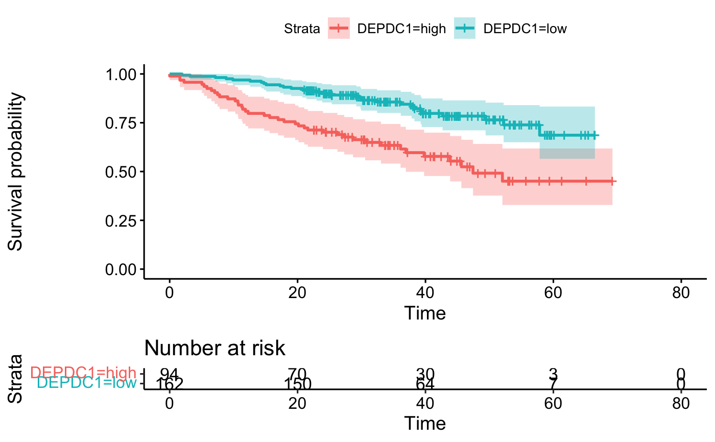
# 4. Fit survival curves and visualize
library("survival")
fit <- survfit(Surv(time, event) ~DEPDC1, data = res.cat)
ggsurvplot(fit, data = res.cat, risk.table = TRUE, conf.int = TRUE)
#> Ignoring unknown labels:
#> • colour : "Strata"
#>
# 3. Categorize variables
res.cat <- surv_categorize(res.cut)
head(res.cat)
#> time event DEPDC1 WHSC1 CRIM1
#> GSM50986 69.24 0 high low high
#> GSM50988 66.43 0 low low low
#> GSM50989 66.50 0 low high high
#> GSM50990 42.67 1 low high low
#> GSM50991 65.00 0 low low low
#> GSM50992 65.20 0 high low low
# 4. Fit survival curves and visualize
library("survival")
fit <- survfit(Surv(time, event) ~DEPDC1, data = res.cat)
ggsurvplot(fit, data = res.cat, risk.table = TRUE, conf.int = TRUE)
#> Ignoring unknown labels:
#> • colour : "Strata"
