
Generic function to create a scatter plot of multivariate analysis outputs, including PCA, CA, MCA and MFA.
Usage
fviz(
  X,
  element,
  axes = c(1, 2),
  geom = "auto",
  label = "all",
  invisible = "none",
  labelsize = 4,
  pointsize = 1.5,
  pointshape = 19,
  arrowsize = 0.5,
  arrow.linetype = "solid",
  habillage = "none",
  addEllipses = FALSE,
  ellipse.level = 0.95,
  ellipse.type = "norm",
  ellipse.alpha = 0.1,
  mean.point = TRUE,
  color = "black",
  fill = "white",
  alpha = 1,
  gradient.cols = NULL,
  col.row.sup = "darkblue",
  col.col.sup = "darkred",
  select = list(name = NULL, cos2 = NULL, contrib = NULL),
  title = NULL,
  axes.linetype = "dashed",
  repel = FALSE,
  col.circle = "grey70",
  circlesize = 0.5,
  add.circle = NULL,
  rotate.labels = FALSE,
  ggtheme = theme_minimal(),
  ggp = NULL,
  font.family = "",
  max.points = NULL,
  sample.seed = 123,
  ...
)
Arguments
- X
an object of class PCA, CA, MCA, FAMD, MFA and HMFA [FactoMineR]; prcomp and princomp [stats]; dudi, pca, coa and acm [ade4]; ca [ca package]; expoOutput [ExPosition].
- element
the element to subset from the output. Possible values are "row" or "col" for CA; "var", "ind", "mca.cor" or "quanti.sup" for MCA; "var" or "ind" for PCA; and 'quanti.var', 'quali.var', 'quali.sup', 'group' or 'ind' for FAMD, MFA and HMFA.
- axes
a numeric vector specifying the axes of interest. Values must be positive integer indices within the available dimensions. Default values are 1:2 for axes 1 and 2.
- geom
a text specifying the geometry to be used for the graph. Default value is "auto". Allowed values are the combination of c("point", "arrow", "text"). Use "point" (to show only points); "text" to show only labels; c("point", "text") or c("arrow", "text") to show both types.
- label
a text specifying the elements to be labelled. Default value is "all". Allowed values are "all", "none", or a combination of c("ind", "ind.sup", "quali", "var", "quanti.sup", "group.sup"). "ind" can be used to label only active individuals. "ind.sup" is for supplementary individuals. "quali" is for supplementary qualitative variables. "var" is for active variables. "quanti.sup" is for quantitative supplementary variables.
- invisible
a text specifying the elements to be hidden on the plot. Default value is "none". Allowed values are "all", "none", or a combination of c("ind", "ind.sup", "quali", "var", "quanti.sup", "group.sup").
- labelsize
font size for the labels
- pointsize
the size of points
- pointshape
the shape of points
- arrowsize
the size of arrows. Controls the thickness of arrows.
- arrow.linetype
linetype of the variable arrows (e.g. "solid", "dashed", "dotted"). Default is "solid".
- habillage
an optional factor variable for coloring the observations by groups. Default value is "none". If X is a PCA object from FactoMineR package, habillage can also specify the supplementary qualitative variable (by its index or name) to be used for coloring individuals by groups (see ?PCA in FactoMineR).
- addEllipses
logical value. If TRUE, draws ellipses around the individuals when habillage != "none".
- ellipse.level
the size of the concentration ellipse in normal probability.
- ellipse.type
Character specifying frame type. Possible values are
"convex","confidence"or types supported bystat_ellipse()including one ofc("t", "norm", "euclid")for plotting concentration ellipses."convex": plot convex hull of a set of points."confidence": plot confidence ellipses around group mean points ascoord.ellipse()[in FactoMineR]."t": assumes a multivariate t-distribution."norm": assumes a multivariate normal distribution."euclid": draws a circle with the radius equal to level, representing the euclidean distance from the center. This ellipse probably won't appear circular unlesscoord_fixed()is applied.
- ellipse.alpha
Alpha for ellipse specifying the transparency level of fill color. Use alpha = 0 for no fill color.
- mean.point
logical value. If TRUE (default), group mean points are added to the plot.
- color
color to be used for the specified geometries (point, text). Can be a continuous variable or a factor variable. Possible values also include "cos2", "contrib", "coord", "x", and "y". In this case, the colors for individuals/variables are automatically controlled by their qualities of representation ("cos2"), contributions ("contrib"), coordinates (x^2+y^2, "coord"), x values ("x") or y values ("y"). To use automatic coloring (by cos2, contrib, ....), make sure that habillage ="none".
- fill
same as the argument
color, but for point fill color. Useful when pointshape = 21, for example.- alpha
controls the transparency of individual and variable colors, respectively. The value can vary from 0 (total transparency) to 1 (no transparency). Default value is 1. Possible values also include "cos2", "contrib", "coord", "x" or "y". In this case, the transparency for the individual/variable colors are automatically controlled by their qualities ("cos2"), contributions ("contrib"), coordinates (x^2+y^2, "coord"), x values("x") or y values("y"). To use this, make sure that habillage ="none".
- gradient.cols
vector of colors to use for n-colour gradient. Allowed values include brewer and ggsci color palettes.
- col.col.sup, col.row.sup
colors for the supplementary column and row points, respectively.
- select
a selection of individuals/variables to be drawn. Allowed values are NULL or a list containing the arguments name, cos2 or contrib:
name: is a character vector containing individuals/variables to be drawn
cos2: if cos2 is in [0, 1], ex: 0.6, then individuals/variables with a cos2 > 0.6 are drawn. if cos2 > 1, ex: 5, then the top 5 individuals/variables with the highest cos2 are drawn.
contrib: if contrib > 1, ex: 5, then the top 5 individuals/variables with the highest contrib are drawn
union: logical. When several of name/cos2/contrib are given, FALSE (default) combines them with AND (each condition further narrows the selection); TRUE combines them with OR (an element is kept if it matches any condition), e.g. named items plus the top-cos2 ones.
- title
the title of the graph
- axes.linetype
linetype of x and y axes.
- repel
logical; whether to use ggrepel to avoid overplotting text labels. The old
jitterargument is kept for backward compatibility and is converted torepel = TRUEwith a deprecation warning.- col.circle
a color for the correlation circle. Used only when X is a PCA output.
- circlesize
the size of the variable correlation circle.
- add.circle
logical or NULL controlling the variable correlation circle. Default NULL shows it only when meaningful: for PCA variables on unit-variance (scaled) data, and for quantitative variables of MCA/MFA/HMFA/FAMD. Use
add.circle = TRUEto force the circle (e.g. aprcomp(scale = FALSE)fit on data you scaled manually) oradd.circle = FALSEto suppress it.- rotate.labels
logical. If
TRUE, the text labels of the plotted element are rotated to the angle of their arrows (ggbiplot style); labels in the left half-plane are flipped to stay upright. Default isFALSE(no rotation). Use together withrepel = FALSE, as ggrepel ignores the label angle. Most useful for variable plots/biplots (e.g.fviz_pca_var,fviz_pca_biplot).- ggtheme
function, ggplot2 theme name. The default is set by each function's
ggthemeargument; see the function usage for the actual default. Setggtheme = NULLto skip applying a ggpubr theme, so the plot keeps ggplot2 default theme or the theme set globally viatheme_set(). Allowed values include ggplot2 official themes: theme_gray(), theme_bw(), theme_minimal(), theme_classic(), theme_void(), ....- ggp
a ggplot. If not NULL, points are added to an existing plot.
- font.family
character vector specifying font family.
- max.points
integer or NULL. When the individual / row / column cloud has more than
max.pointspoints, a random subset of that many points is drawn so the plot stays readable (usable labels instead of an over-plotted cloud). Only the drawn points/labels are thinned: any ellipse (addEllipses) and the group mean point are still computed on the full data, so a convex / confidence frame is not shrunk or inflated by the draw. When points are coloured/split by a group (e.g.habillage), the draw is stratified so every group keeps at least a minimum number of points and none is decimated. When colour, fill or size is mapped to a continuous metric (e.g.col.ind = "cos2"), its scale and legend are pinned to the full-data range, so a point's colour, fill and size do not depend on how many points are drawn. A message reports how many points are shown. The subset is reproducible (seesample.seed) and does not change the caller's random stream.NULL(default) draws every point.- sample.seed
the random seed used to pick the
max.pointssubset, for a reproducible figure. Ignored whenmax.pointsisNULL.- ...
Arguments to be passed to the functions ggpubr::ggscatter() & ggpubr::ggpar().
Author
Alboukadel Kassambara alboukadel.kassambara@gmail.com
Examples
# \donttest{
# Principal component analysis
# +++++++++++++++++++++++++++++
data(decathlon2)
decathlon2.active <- decathlon2[1:23, 1:10]
res.pca <- prcomp(decathlon2.active, scale = TRUE)
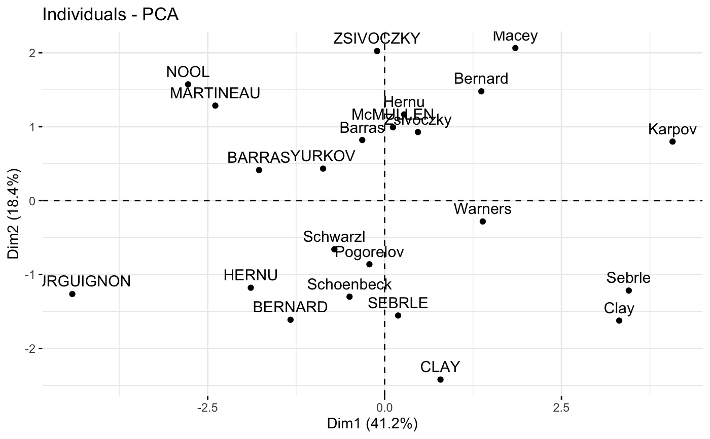
fviz(res.pca, "ind") # Individuals plot
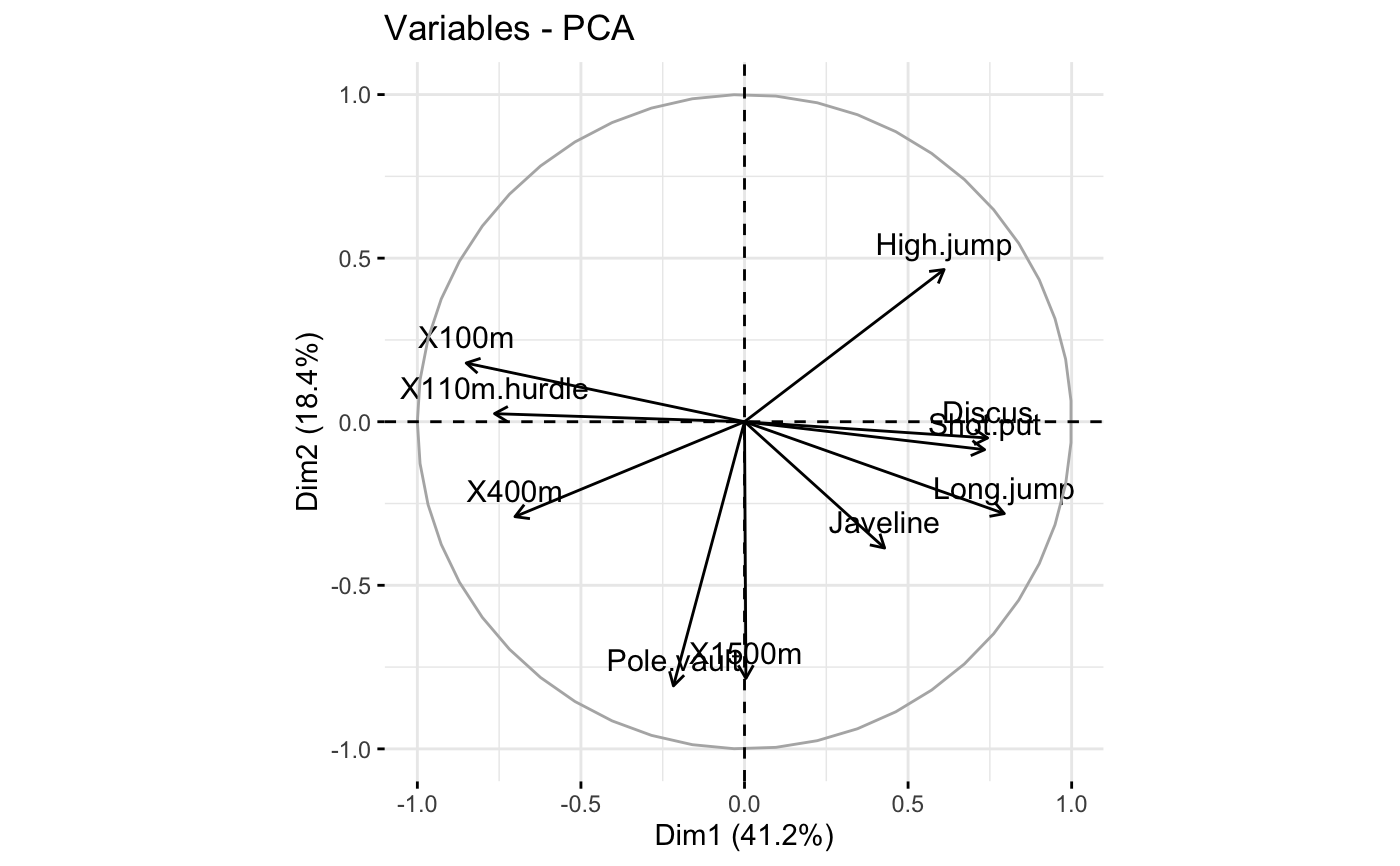
 fviz(res.pca, "var") # Variables plot
 # Correspondence Analysis
# ++++++++++++++++++++++++++
# Install and load FactoMineR to compute CA
# install.packages("FactoMineR")
library("FactoMineR")
data("housetasks")
res.ca <- CA(housetasks, graph = FALSE)
fviz(res.ca, "row") # Rows plot
# Correspondence Analysis
# ++++++++++++++++++++++++++
# Install and load FactoMineR to compute CA
# install.packages("FactoMineR")
library("FactoMineR")
data("housetasks")
res.ca <- CA(housetasks, graph = FALSE)
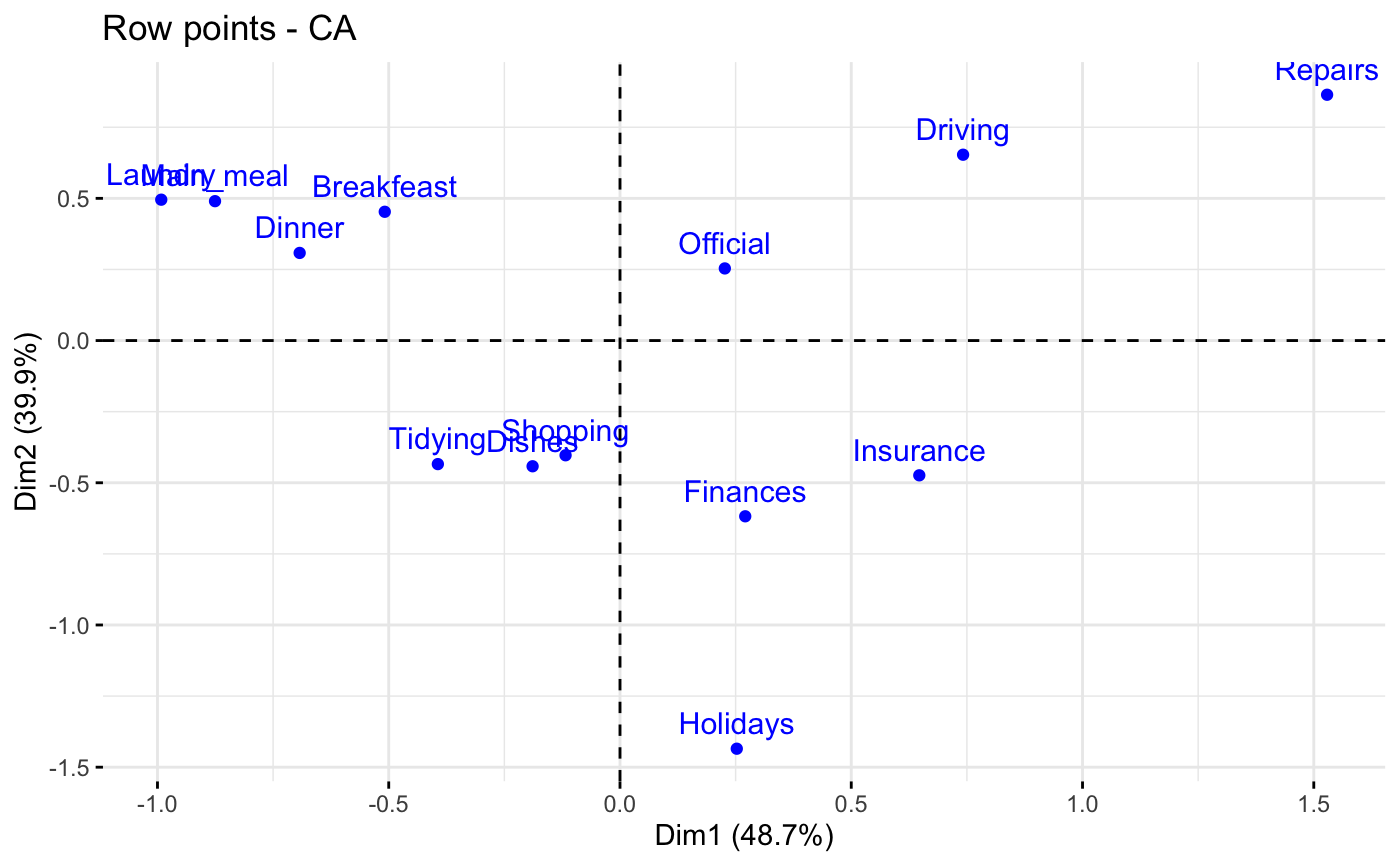
fviz(res.ca, "row") # Rows plot
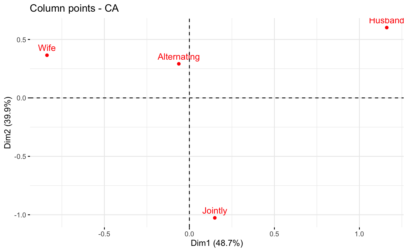
 fviz(res.ca, "col") # Columns plot
 # Multiple Correspondence Analysis
# +++++++++++++++++++++++++++++++++
library(FactoMineR)
data(poison)
res.mca <- MCA(poison, quanti.sup = 1:2,
quali.sup = 3:4, graph=FALSE)
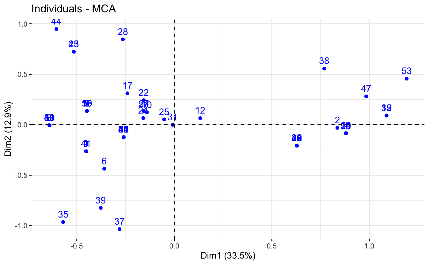
fviz(res.mca, "ind") # Individuals plot
# Multiple Correspondence Analysis
# +++++++++++++++++++++++++++++++++
library(FactoMineR)
data(poison)
res.mca <- MCA(poison, quanti.sup = 1:2,
quali.sup = 3:4, graph=FALSE)
fviz(res.mca, "ind") # Individuals plot
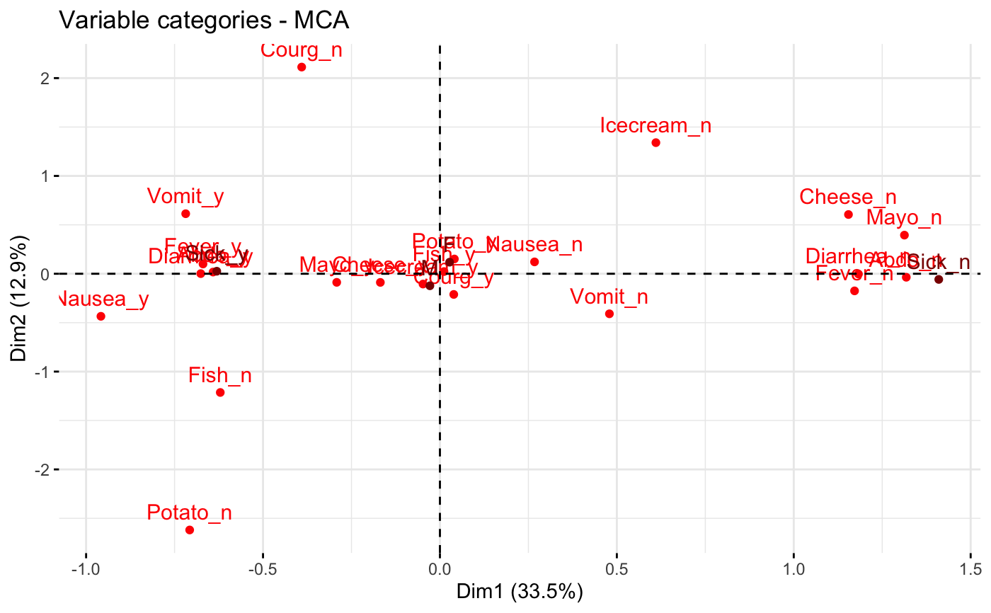
 fviz(res.mca, "var") # Variables plot
 # }
# }