
Eigenvalues correspond to the amount of the variation explained by each principal component (PC).
get_eig(): Extract the eigenvalues/variances of the principal dimensions
fviz_eig(): Plot the eigenvalues/variances against the number of dimensions
get_eigenvalue(): an alias of get_eig()
fviz_screeplot(): an alias of fviz_eig()
These functions support the results of Principal Component Analysis (PCA),
Correspondence Analysis (CA), Multiple Correspondence Analysis (MCA), Factor Analysis of Mixed Data (FAMD),
Multiple Factor Analysis (MFA) and Hierarchical Multiple Factor Analysis
(HMFA) functions. fviz_eig() validates ncp,
parallel.iter, and parallel.seed before plotting, accepting
integer-like numeric values while still rejecting fractional inputs.
Recent versions of FactoMineR::PCA() may retain only the number of
eigenvalues requested through its ncp argument. When the stored
eigenvalues do not account for the result's recorded total inertia,
fviz_eig() warns that the scree plot is incomplete. Refit the PCA
with a sufficiently large ncp to plot the complete spectrum.
get_eig() continues to return the eigenvalues stored in the object.
Read more: Principal Component Analysis (PCA) in R: Compute, Visualize & Interpret.
Usage
get_eig(X)

get_eigenvalue(X)

fviz_eig(
  X,
  choice = c("variance", "eigenvalue"),
  geom = c("bar", "line"),
  barfill = "steelblue",
  barcolor = "steelblue",
  linecolor = "black",
  ncp = 10,
  addlabels = FALSE,
  hjust = 0,
  main = NULL,
  xlab = NULL,
  ylab = NULL,
  ggtheme = theme_minimal(),
  parallel = FALSE,
  parallel.color = "red",
  parallel.lty = "dashed",
  parallel.iter = 100,
  parallel.seed = NULL,
  ...
)

fviz_screeplot(...)
Arguments
- X
an object of class PCA, CA, MCA, FAMD, MFA, or HMFA [FactoMineR];
prcomporprincomp[stats];factoextra_pca;dudi,pca,coa,acm,between, orwithin[ade4];caormjca[ca];correspondence[MASS]; orexpoOutput[ExPosition].- choice
a text specifying the data to be plotted. Allowed values are "variance" or "eigenvalue".
- geom
a text specifying the geometry to be used for the graph. Allowed values are "bar" for barplot, "line" for lineplot or c("bar", "line") to use both types.
- barfill
fill color for bar plot.
- barcolor
outline color for bar plot.
- linecolor
color for line plot (when geom contains "line").
- ncp
a single positive integer specifying the number of dimensions to be shown. Integer-like numeric values are accepted.
- addlabels
logical value. If TRUE, labels are added at the top of bars or points showing the information retained by each dimension.
- hjust
horizontal adjustment of the labels.
- main, xlab, ylab
plot main and axis titles.
- ggtheme
function, ggplot2 theme name. The default is set by each function's
ggthemeargument; see the function usage for the actual default. Setggtheme = NULLto skip applying a ggpubr theme, so the plot keeps ggplot2 default theme or the theme set globally viatheme_set(). Allowed values include ggplot2 official themes: theme_gray(), theme_bw(), theme_minimal(), theme_classic(), theme_void(), ....- parallel
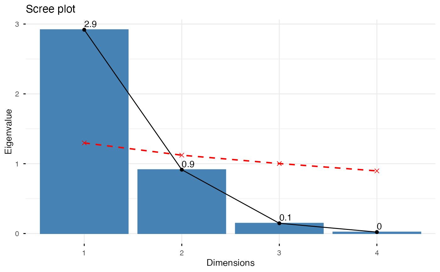
logical value. If TRUE, adds a Horn parallel-analysis threshold curve. Each point is the 95th percentile of the corresponding ordered eigenvalue from independently simulated reference data. Components whose eigenvalues exceed their component-specific thresholds are retained by the parallel-analysis rule. Correlation PCA uses standardized reference data; covariance PCA uses reconstructed marginal scales. This is available only when
choice = "eigenvalue"andXis a sufficiently completeprcomporprincompobject. Mean centering is required;prcompalso requires retained scores. Custom scaling and incomplete covariance decompositions are rejected when their reference distribution cannot be reconstructed. Default is FALSE.- parallel.color
color of the parallel-analysis threshold curve. Default is "red".
- parallel.lty
line type for the parallel-analysis curve. Default is "dashed".
- parallel.iter
a single positive integer giving the number of iterations for parallel analysis simulation. Integer-like numeric values are accepted. Default is 100.
- parallel.seed
NULL or a single non-negative integer seed for reproducible parallel analysis simulation. If NULL (default), the current RNG stream is used. Integer-like numeric values are accepted.
- ...
optional arguments to be passed to the function ggpar.
Value
get_eig() (or get_eigenvalue()): returns a data.frame containing 3 columns: the eigenvalues, the percentage of variance and the cumulative percentage of variance retained by each dimension.
fviz_eig() (or fviz_screeplot()): returns a ggplot2
Author
Alboukadel Kassambara alboukadel.kassambara@gmail.com
Examples
# Principal Component Analysis
# ++++++++++++++++++++++++++
data(iris)
res.pca <- prcomp(iris[, -5], scale = TRUE)
# Extract eigenvalues/variances
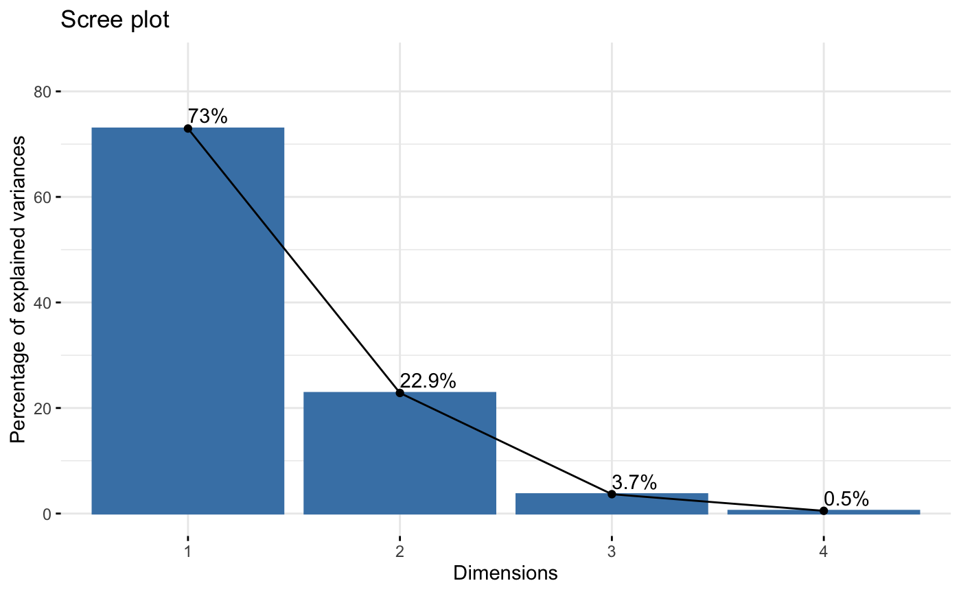
get_eig(res.pca)
#> eigenvalue variance.percent cumulative.variance.percent
#> Dim.1 2.91849782 72.9624454 72.96245
#> Dim.2 0.91403047 22.8507618 95.81321
#> Dim.3 0.14675688 3.6689219 99.48213
#> Dim.4 0.02071484 0.5178709 100.00000
# Default plot
fviz_eig(res.pca, addlabels = TRUE, ylim = c(0, 85))
 # Scree plot - Eigenvalues
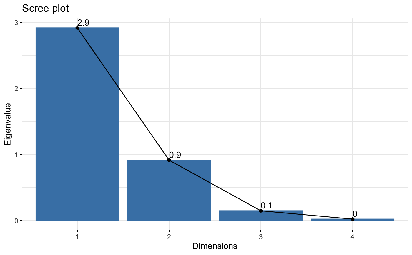
fviz_eig(res.pca, choice = "eigenvalue", addlabels=TRUE)
# Scree plot - Eigenvalues
fviz_eig(res.pca, choice = "eigenvalue", addlabels=TRUE)
 # Use only bar or line plot: geom = "bar" or geom = "line"
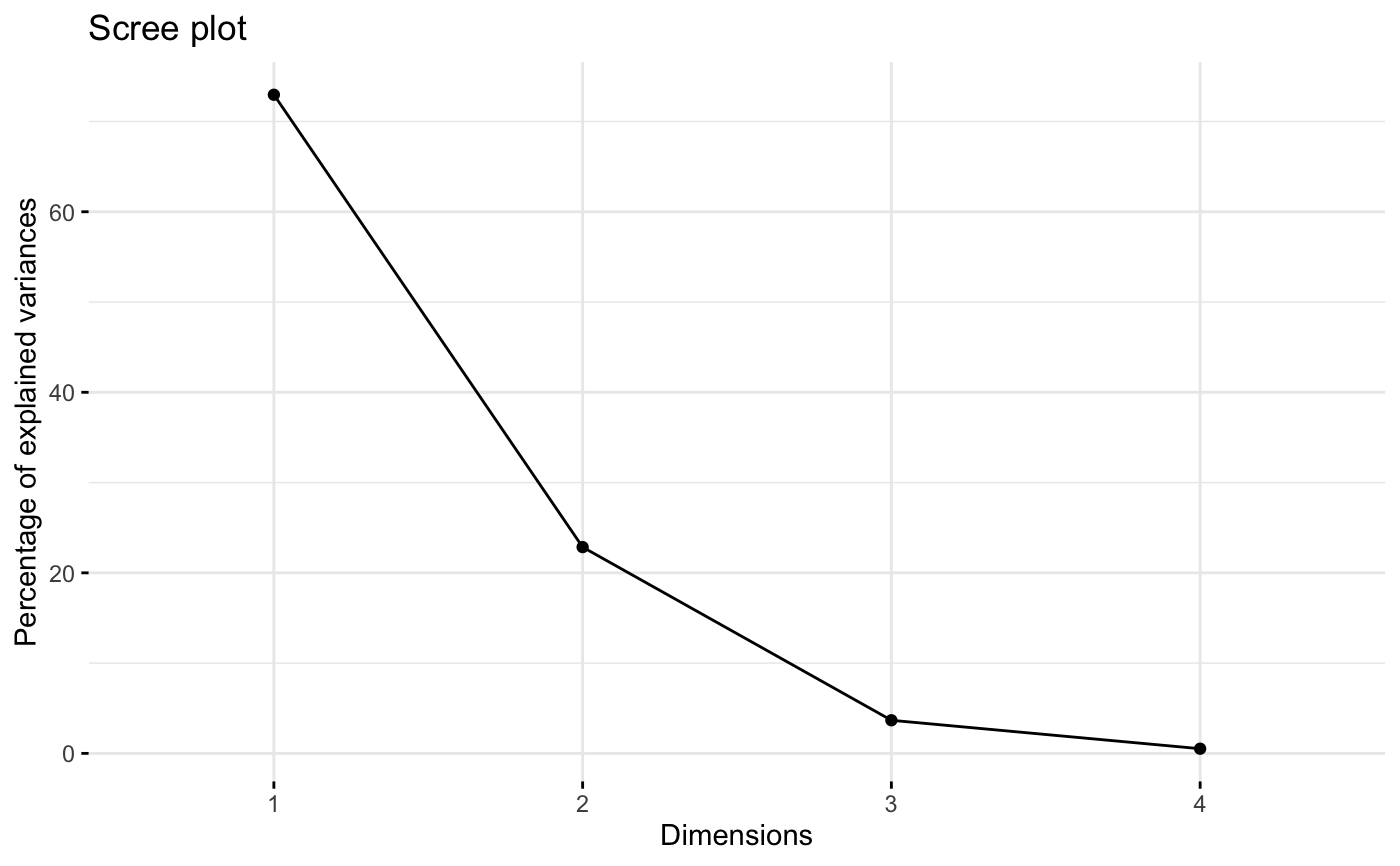
fviz_eig(res.pca, geom="line")
# Use only bar or line plot: geom = "bar" or geom = "line"
fviz_eig(res.pca, geom="line")
 # Parallel analysis (Horn's method) to determine the number of components
# Retain components whose eigenvalues exceed their component-specific points
fviz_eig(res.pca, choice = "eigenvalue", parallel = TRUE,
addlabels = TRUE, parallel.color = "red",
parallel.iter = 10, parallel.seed = 123)
# Parallel analysis (Horn's method) to determine the number of components
# Retain components whose eigenvalues exceed their component-specific points
fviz_eig(res.pca, choice = "eigenvalue", parallel = TRUE,
addlabels = TRUE, parallel.color = "red",
parallel.iter = 10, parallel.seed = 123)
 if (FALSE) { # \dontrun{
# Correspondence Analysis
# +++++++++++++++++++++++++++++++++
library(FactoMineR)
data(housetasks)
res.ca <- CA(housetasks, graph = FALSE)
get_eig(res.ca)
fviz_eig(res.ca, linecolor = "#FC4E07",
barcolor = "#00AFBB", barfill = "#00AFBB")
# Multiple Correspondence Analysis
# +++++++++++++++++++++++++++++++++
library(FactoMineR)
data(poison)
res.mca <- MCA(poison, quanti.sup = 1:2,
quali.sup = 3:4, graph=FALSE)
get_eig(res.mca)
fviz_eig(res.mca, linecolor = "#FC4E07",
barcolor = "#2E9FDF", barfill = "#2E9FDF")
} # }
if (FALSE) { # \dontrun{
# Correspondence Analysis
# +++++++++++++++++++++++++++++++++
library(FactoMineR)
data(housetasks)
res.ca <- CA(housetasks, graph = FALSE)
get_eig(res.ca)
fviz_eig(res.ca, linecolor = "#FC4E07",
barcolor = "#00AFBB", barfill = "#00AFBB")
# Multiple Correspondence Analysis
# +++++++++++++++++++++++++++++++++
library(FactoMineR)
data(poison)
res.mca <- MCA(poison, quanti.sup = 1:2,
quali.sup = 3:4, graph=FALSE)
get_eig(res.mca)
fviz_eig(res.mca, linecolor = "#FC4E07",
barcolor = "#2E9FDF", barfill = "#2E9FDF")
} # }