
This function can be used to visualize the quality of representation (cos2) of rows/columns from the results of Principal Component Analysis (PCA), Correspondence Analysis (CA), Multiple Correspondence Analysis (MCA), Factor Analysis of Mixed Data (FAMD), Multiple Factor Analysis (MFA) and Hierarchical Multiple Factor Analysis (HMFA) functions.
Read more: Principal Component Analysis (PCA) in R: Compute, Visualize & Interpret.
Usage
fviz_cos2(
  X,
  choice = c("row", "col", "var", "ind", "quanti.var", "quali.var", "group"),
  axes = 1,
  fill = "steelblue",
  color = "steelblue",
  sort.val = c("desc", "asc", "none"),
  top = Inf,
  xtickslab.rt = 45,
  ggtheme = theme_minimal(),
  display = c("bar", "heatmap"),
  ...
)
Arguments
- X
an object of class PCA, CA, MCA, FAMD, MFA and HMFA [FactoMineR]; prcomp and princomp [stats]; dudi, pca, coa and acm [ade4]; ca [ca package].
- choice
allowed values are "row" and "col" for CA; "var" and "ind" for PCA or MCA; "var", "ind", "quanti.var", "quali.var" and "group" for FAMD, MFA and HMFA.
- axes
a numeric vector specifying the dimension(s) of interest.
- fill
a fill color for the bar plot.
- color
an outline color for the bar plot.
- sort.val
a string specifying whether the value should be sorted. Allowed values are "none" (no sorting), "asc" (for ascending) or "desc" (for descending).
- top
a numeric value specifying the number of top elements to be shown.
- xtickslab.rt
rotation angle for x axis tick labels. Default is 45 degrees.
- ggtheme
function, ggplot2 theme name. The default is set by each function's
ggthemeargument; see the function usage for the actual default. Setggtheme = NULLto skip applying a ggpubr theme, so the plot keeps ggplot2 default theme or the theme set globally viatheme_set(). Allowed values include ggplot2 official themes: theme_gray(), theme_bw(), theme_minimal(), theme_classic(), theme_void(), ....- display
how to display the values.
"bar"(default) draws the usual barplot of the cos2/contribution summed overaxes."heatmap"draws a grid with one tile per element and dimension, filled by the per-dimension cos2/contribution and labelled with its value, so several dimensions can be read at once. With"heatmap", elements are ordered by their (unweighted) total over the requestedaxesandtopkeeps the leading ones; the bar-specificsort.valandcolorarguments are ignored, andfillsets the high end of the white-to-colour gradient.- ...
not used
Author
Alboukadel Kassambara alboukadel.kassambara@gmail.com
Examples
# \donttest{
# Principal component analysis
# ++++++++++++++++++++++++++
data(decathlon2)
decathlon2.active <- decathlon2[1:23, 1:10]
res.pca <- prcomp(decathlon2.active, scale = TRUE)
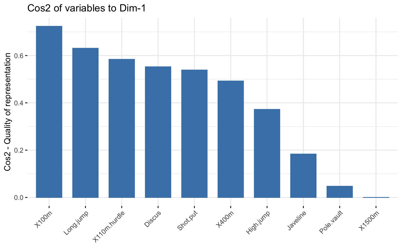
# variable cos2 on axis 1
fviz_cos2(res.pca, choice="var", axes = 1, top = 10 )
 # Change color
fviz_cos2(res.pca, choice="var", axes = 1,
fill = "lightgray", color = "black")
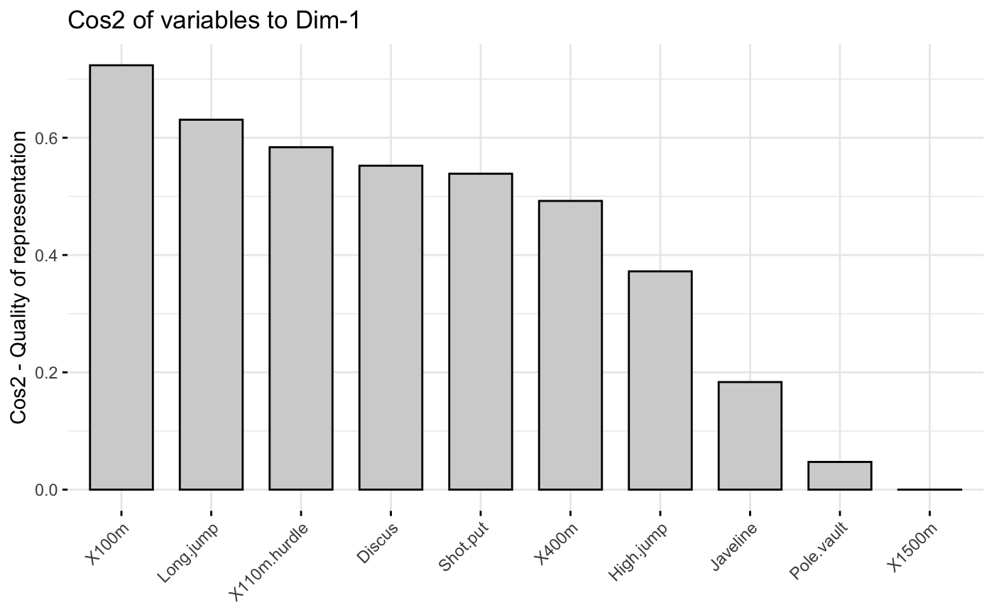
# Change color
fviz_cos2(res.pca, choice="var", axes = 1,
fill = "lightgray", color = "black")
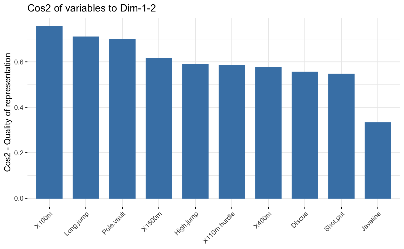
 # Variable cos2 on axes 1 + 2
fviz_cos2(res.pca, choice="var", axes = 1:2)
# Variable cos2 on axes 1 + 2
fviz_cos2(res.pca, choice="var", axes = 1:2)
 # Heat-grid of cos2 across several dimensions
fviz_cos2(res.pca, choice = "var", axes = 1:4, display = "heatmap")
# Heat-grid of cos2 across several dimensions
fviz_cos2(res.pca, choice = "var", axes = 1:4, display = "heatmap")
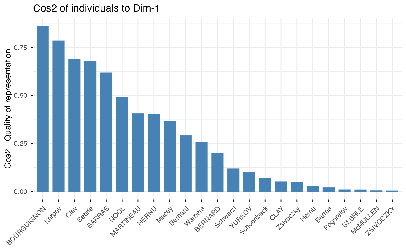
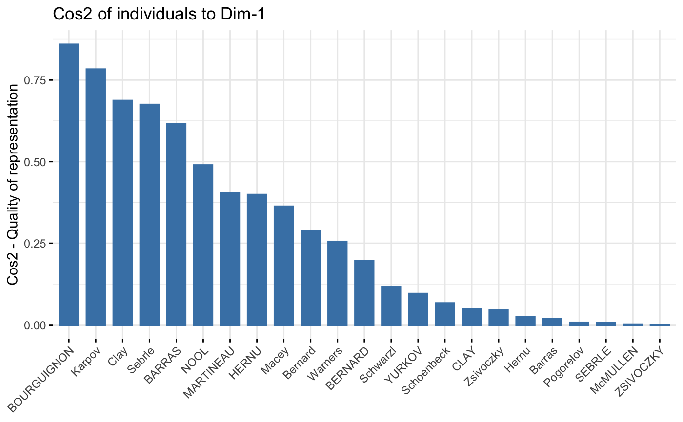 # cos2 of individuals on axis 1
fviz_cos2(res.pca, choice="ind", axes = 1)
# cos2 of individuals on axis 1
fviz_cos2(res.pca, choice="ind", axes = 1)
 if (FALSE) { # \dontrun{
# Correspondence Analysis
# ++++++++++++++++++++++++++
library("FactoMineR")
data("housetasks")
res.ca <- CA(housetasks, graph = FALSE)
# Visualize row cos2 on axes 1
fviz_cos2(res.ca, choice ="row", axes = 1)
# Visualize column cos2 on axes 1
fviz_cos2(res.ca, choice ="col", axes = 1)
# Multiple Correspondence Analysis
# +++++++++++++++++++++++++++++++++
library(FactoMineR)
data(poison)
res.mca <- MCA(poison, quanti.sup = 1:2,
quali.sup = 3:4, graph=FALSE)
# Visualize individual cos2 on axes 1
fviz_cos2(res.mca, choice ="ind", axes = 1, top = 20)
# Visualize variable category cos2 on axes 1
fviz_cos2(res.mca, choice ="var", axes = 1)
# Multiple Factor Analysis
# ++++++++++++++++++++++++
library(FactoMineR)
data(poison)
res.mfa <- MFA(poison, group=c(2,2,5,6), type=c("s","n","n","n"),
name.group=c("desc","desc2","symptom","eat"),
num.group.sup=1:2, graph=FALSE)
# Visualize individual cos2 on axes 1
# Select the top 20
fviz_cos2(res.mfa, choice ="ind", axes = 1, top = 20)
# Visualize categorical variable category cos2 on axes 1
fviz_cos2(res.mfa, choice ="quali.var", axes = 1)
} # }
# }
if (FALSE) { # \dontrun{
# Correspondence Analysis
# ++++++++++++++++++++++++++
library("FactoMineR")
data("housetasks")
res.ca <- CA(housetasks, graph = FALSE)
# Visualize row cos2 on axes 1
fviz_cos2(res.ca, choice ="row", axes = 1)
# Visualize column cos2 on axes 1
fviz_cos2(res.ca, choice ="col", axes = 1)
# Multiple Correspondence Analysis
# +++++++++++++++++++++++++++++++++
library(FactoMineR)
data(poison)
res.mca <- MCA(poison, quanti.sup = 1:2,
quali.sup = 3:4, graph=FALSE)
# Visualize individual cos2 on axes 1
fviz_cos2(res.mca, choice ="ind", axes = 1, top = 20)
# Visualize variable category cos2 on axes 1
fviz_cos2(res.mca, choice ="var", axes = 1)
# Multiple Factor Analysis
# ++++++++++++++++++++++++
library(FactoMineR)
data(poison)
res.mfa <- MFA(poison, group=c(2,2,5,6), type=c("s","n","n","n"),
name.group=c("desc","desc2","symptom","eat"),
num.group.sup=1:2, graph=FALSE)
# Visualize individual cos2 on axes 1
# Select the top 20
fviz_cos2(res.mfa, choice ="ind", axes = 1, top = 20)
# Visualize categorical variable category cos2 on axes 1
fviz_cos2(res.mfa, choice ="quali.var", axes = 1)
} # }
# }