
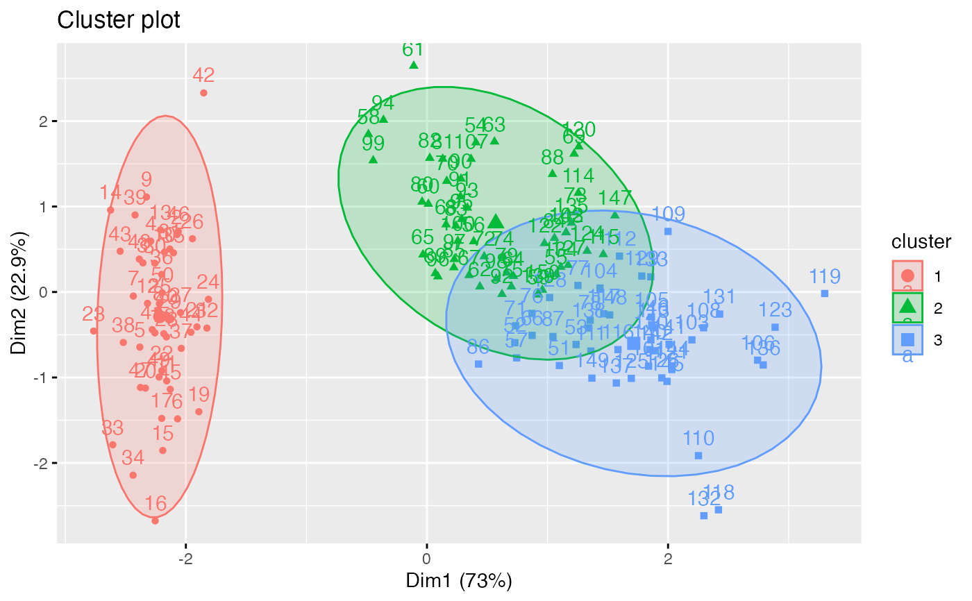
Provides ggplot2-based elegant visualization of partitioning
methods including kmeans [stats package]; pam, clara and fanny [cluster
package]; dbscan [fpc package]; Mclust [mclust package]; HCPC [FactoMineR];
hkmeans [factoextra]. Observations are represented by points in the plot,
using principal components if ncol(data) > 2. An ellipse is drawn around
each cluster. When stand = TRUE, the plotting data must remain
finite after scaling.
Read more: K-Means Clustering in R: Algorithm, Visualization & Interpretation.
Usage
fviz_cluster(
  object,
  data = NULL,
  choose.vars = NULL,
  stand = TRUE,
  axes = c(1, 2),
  geom = c("point", "text"),
  repel = FALSE,
  show.clust.cent = TRUE,
  ellipse = TRUE,
  ellipse.type = "convex",
  ellipse.level = 0.95,
  ellipse.alpha = 0.2,
  shape = NULL,
  pointsize = 1.5,
  labelsize = 12,
  main = "Cluster plot",
  xlab = NULL,
  ylab = NULL,
  outlier.color = "black",
  outlier.shape = 19,
  outlier.pointsize = pointsize,
  outlier.labelsize = labelsize,
  ggtheme = theme_grey(),
  max.points = NULL,
  sample.seed = 123,
  ...
)
Arguments
- object
an object of class "partition" created by
pam(),clara(), orfanny()[cluster]; "kmeans" [stats]; "dbscan" [fpc]; "Mclust" [mclust]; or "hkmeans" or "eclust" [factoextra]. A custom list may instead containdataplus eitherclusterorclustering. When the assignments and the data both carry complete, unique, matching names, the assignments are aligned to the data rows by name; otherwise they are used in their given (positional) order. The exception is a clustering fitted from dissimilarities and plotted with externaldata: complete, unique, non-matching name sets are rejected because positional use would attach clusters to the wrong observations.- data
the data used for clustering. It is required for kmeans and dbscan objects, and for partition or hcut objects fitted from dissimilarities when those objects do not retain the original observations.
- choose.vars
a character vector containing variables to be considered for plotting.
- stand
logical value; if TRUE, data is standardized before principal component analysis. If scaling produces
NAvalues,fviz_cluster()stops with a package-level error.- axes
a numeric vector of length 2 specifying the dimensions to be plotted.
- geom
a text specifying the geometry to be used for the graph. Allowed values are the combination of c("point", "text"). Use "point" (to show only points); "text" to show only labels; c("point", "text") to show both types.
- repel
logical; whether to use ggrepel to avoid overplotting text labels. The old
jitterargument is kept for backward compatibility and is converted torepel = TRUEwith a deprecation warning.- show.clust.cent
logical; if TRUE, shows cluster centers
- ellipse
logical value; if TRUE, draws outline around points of each cluster
- ellipse.type
Character specifying frame type. Possible values are 'convex', 'confidence' or types supported by
stat_ellipseincluding one of c("t", "norm", "euclid").- ellipse.level
the size of the concentration ellipse in normal probability. Passed for
ggplot2::stat_ellipse's level. Ignored in 'convex'. Default value is 0.95.- ellipse.alpha
Alpha for frame specifying the transparency level of fill color. Use alpha = 0 for no fill color.
- shape
the shape of points.
- pointsize
the size of points
- labelsize
font size for the labels
- main
plot main title.
- xlab, ylab
character vector specifying x and y axis labels, respectively. Use xlab = FALSE and ylab = FALSE to hide xlab and ylab, respectively.
- outlier.pointsize, outlier.color, outlier.shape, outlier.labelsize
arguments for customizing outliers, which can be detected only in DBSCAN clustering.
- ggtheme
function, ggplot2 theme name. The default is set by each function's
ggthemeargument; see the function usage for the actual default. Setggtheme = NULLto skip applying a ggpubr theme, so the plot keeps ggplot2 default theme or the theme set globally viatheme_set(). Allowed values include ggplot2 official themes: theme_gray(), theme_bw(), theme_minimal(), theme_classic(), theme_void(), ....- max.points
integer or NULL. When the data has more than
max.pointsobservations, a random subset of that many points is drawn so the cluster plot stays readable instead of over-plotting. Only the drawn scatter/labels are thinned: the cluster frame (convex hull / ellipse) and centres are still computed on the full data, so a convex hull is not shrunk by dropping the extreme points a random draw tends to lose. The draw is stratified by cluster so every cluster keeps at least a minimum number of points, and a message reports how many are shown. Any DBSCAN/Mclust outliers are always drawn. The subset is reproducible (seesample.seed) and does not change the caller's random stream.NULL(default) draws every observation.- sample.seed
the random seed used to pick the
max.pointssubset, for a reproducible figure. Ignored whenmax.pointsisNULL.- ...
other arguments to be passed to the functions
ggscatterandggpar.
See also
fviz_silhouette, hcut,
hkmeans, eclust, fviz_dend.
Online tutorial: K-Means Clustering in R: Algorithm, Visualization & Interpretation.
Author
Alboukadel Kassambara alboukadel.kassambara@gmail.com
Examples
set.seed(123)
# Data preparation
# +++++++++++++++
data("iris")
head(iris)
#> Sepal.Length Sepal.Width Petal.Length Petal.Width Species
#> 1 5.1 3.5 1.4 0.2 setosa
#> 2 4.9 3.0 1.4 0.2 setosa
#> 3 4.7 3.2 1.3 0.2 setosa
#> 4 4.6 3.1 1.5 0.2 setosa
#> 5 5.0 3.6 1.4 0.2 setosa
#> 6 5.4 3.9 1.7 0.4 setosa
# Remove species column (5) and scale the data
iris.scaled <- scale(iris[, -5])
# K-means clustering
# +++++++++++++++++++++
km.res <- kmeans(iris.scaled, 3, nstart = 10)
# Visualize kmeans clustering
# use repel = TRUE to avoid overplotting
fviz_cluster(km.res, iris[, -5], ellipse.type = "norm")
 # Change the color palette and theme
fviz_cluster(km.res, iris[, -5],
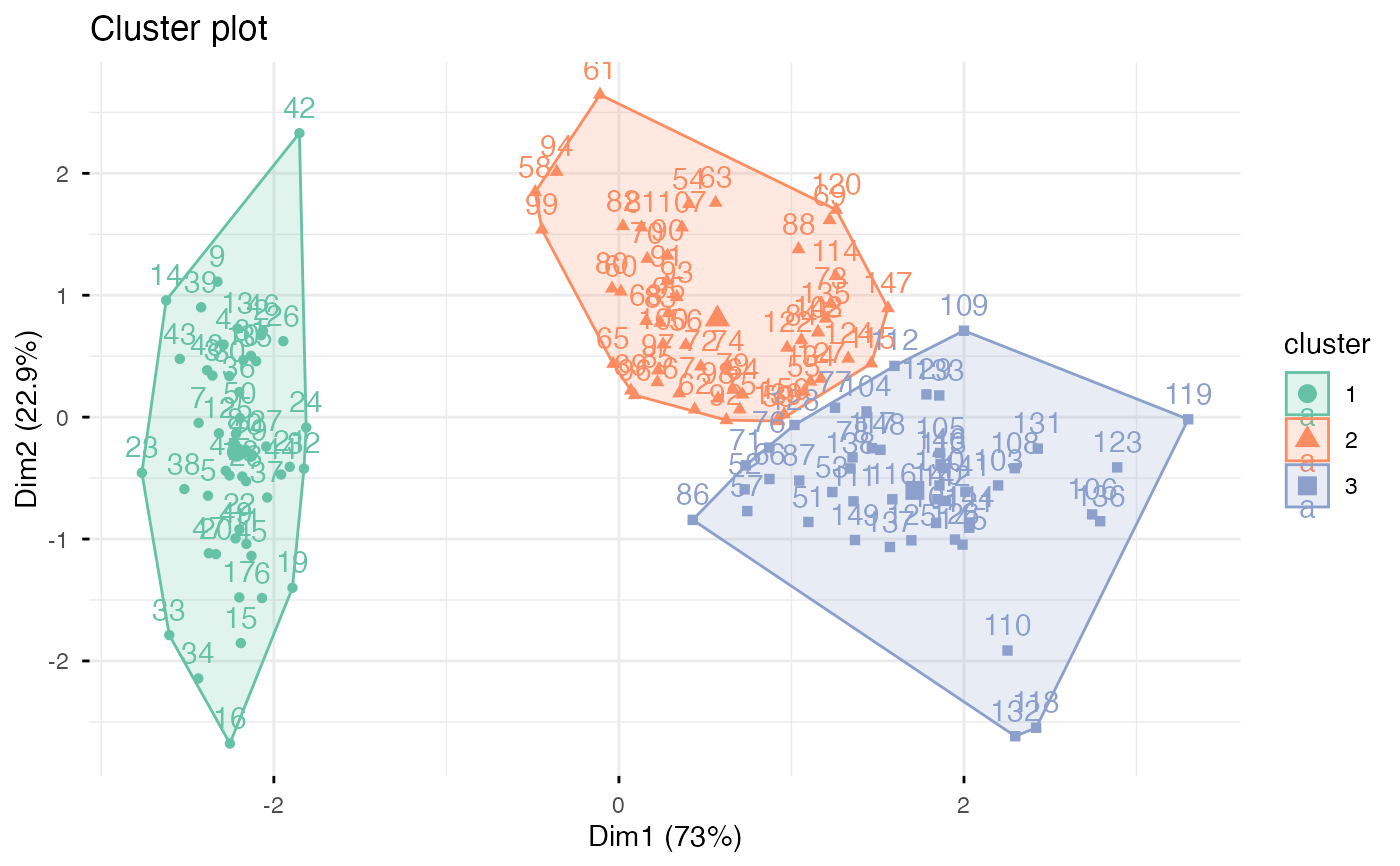
palette = "Set2", ggtheme = theme_minimal())
# Change the color palette and theme
fviz_cluster(km.res, iris[, -5],
palette = "Set2", ggtheme = theme_minimal())
 if (FALSE) { # \dontrun{
# Show points only
fviz_cluster(km.res, iris[, -5], geom = "point")
# Show text only
fviz_cluster(km.res, iris[, -5], geom = "text")
# PAM clustering
# ++++++++++++++++++++
requireNamespace("cluster", quietly = TRUE)
pam.res <- cluster::pam(iris.scaled, 3)
# Visualize pam clustering
fviz_cluster(pam.res, geom = "point", ellipse.type = "norm")
# Hierarchical clustering
# ++++++++++++++++++++++++
# Use hcut(), which computes hclust and cuts the tree
hc.cut <- hcut(iris.scaled, k = 3, hc_method = "complete")
# Visualize dendrogram
fviz_dend(hc.cut, show_labels = FALSE, rect = TRUE)
# Visualize cluster
fviz_cluster(hc.cut, ellipse.type = "convex")
} # }
if (FALSE) { # \dontrun{
# Show points only
fviz_cluster(km.res, iris[, -5], geom = "point")
# Show text only
fviz_cluster(km.res, iris[, -5], geom = "text")
# PAM clustering
# ++++++++++++++++++++
requireNamespace("cluster", quietly = TRUE)
pam.res <- cluster::pam(iris.scaled, 3)
# Visualize pam clustering
fviz_cluster(pam.res, geom = "point", ellipse.type = "norm")
# Hierarchical clustering
# ++++++++++++++++++++++++
# Use hcut(), which computes hclust and cuts the tree
hc.cut <- hcut(iris.scaled, k = 3, hc_method = "complete")
# Visualize dendrogram
fviz_dend(hc.cut, show_labels = FALSE, rect = TRUE)
# Visualize cluster
fviz_cluster(hc.cut, ellipse.type = "convex")
} # }